Fichièr:Equipotential by Zureks.png

Talha d'aquesta previsualizacion: 366 × 600 pixèls. Autras resolucions : 146 × 240 pixèls | 639 × 1 047 pixèls.
Fichièr d'origina (639 × 1 047 pixèl, talha del fichièr: 111 Ko, tipe MIME: image/png)
| Aqueste fichièr proven de Wikimedia Commons?. Las informacions que lo concernisson son afichadas çaijós (procedura). |
Descripcion
| Descripcion |
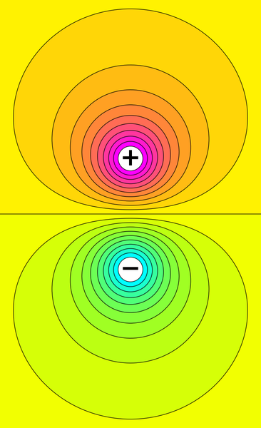
English: Voltage distribution between two electrically charged spheres (purple = positive voltage, blue = negative voltage). The black curves show equipotential contours. |
|||
| Data | ||||
| Font | Trabalh personal | |||
| Autor | Zureks | |||
| Autras versions |
|


Source code
The image can be created with Python Matplotlib using the following code:
import numpy as np
from matplotlib import pyplot as plt
from matplotlib import colors

cmap = colors.ListedColormap([np.clip((2*x, 2*(1-x), 4*(x-0.5)**2), 0, 1) for x in np.linspace(0., 1., 256)])

w, h = 639, 1047
xmax = 2.36
ymax = xmax * float(h) / float(w)
vmax = 0.78
y0 = 1.0
nlevels = 21
levels = np.linspace(-vmax, vmax, nlevels)
X, Y = np.mgrid[-xmax:xmax:250j, -ymax:ymax:800j]

# potential of two point charges
V  = 1.0 / np.maximum(np.sqrt(X**2 + (Y - y0)**2), 1e-2)
V -= 1.0 / np.maximum(np.sqrt(X**2 + (Y + y0)**2), 1e-2)

# rescale potential globally to make contour areas similar
V = (np.sqrt(1 + V * V) - 1) / V

plt.figure(figsize=(w/90., h/90.)).add_axes([0, 0, 1, 1])
contf = plt.contourf(X, Y, V, levels=levels, cmap=cmap,
         vmin=-vmax*(nlevels-1.)/nlevels, vmax=vmax*(nlevels-1.)/nlevels)
cont = plt.contour(X, Y, V, levels=contf.levels, colors='k', linestyles='solid')

plt.xticks([]), plt.yticks([])
plt.gca().set_aspect(aspect='equal')
plt.gca().axis('off')
plt.text(0, -y0, u'\u2212', size=48,fontweight='bold', ha='center', va='center')
plt.text(0, y0, '+', size=48,fontweight='bold', ha='center', va='center')
plt.savefig('Equipotential_of_dipole.png')
Publicat jos licéncia(s)
| L'ús d'aquest fitxer és regulat sota les condicions de Creative Commons de CC0 1.0 lliurament al domini públic universal. | |
| La persona que ha associat un treball amb aquest document ha dedicat l'obra domini públic, renunciant en tot el món a tots els seus drets de d'autor i a tots els drets legals relacionats que tenia en l'obra, en la mesura permesa per la llei. Podeu copiar, modificar, distribuir i modificar l'obra, fins i tot amb fins comercials, tot sense demanar permís.
|
Istoric del fichièr
Clicar sus una data e una ora per veire lo fichièr tal coma èra a aqueste moment
| Data e ora | Miniatura | Dimensions | Utilizaire | Comentari | |
|---|---|---|---|---|---|
| actual | 16 mai de 2018 a 21.09 | | 639×1 047 (111 Ko) | Geek3 | Replaced with analytically computed precise contour shapes. The old version which came from an FEM simulation had significant errors towards the edges, possibly because the simulation volume was chosen too small. The potential dropped much too slowly towards the image edges. In contrast, the analytic solution is very simple, as the potential is just the linear sum of two 1/r potentials. |
| 11 abril de 2010 a 16.37 |  | 639×1 047 (32 Ko) | Zureks | {{Information |Description={{en|1=Voltage distribution between two electrically charged spheres (purple = positive voltage, blue = negative voltage). The black curves show equipotential contours.}} |Source={{own}} |Author=Zureks |Date=2010 |
Paginas que contenon lo fichièr
La pagina çaijós compòrta aqueste imatge :
Usatge global del fichièr
Los autres wikis seguents utilizan aqueste imatge :
- Utilizacion sus ar.wikipedia.org
- Utilizacion sus be-tarask.wikipedia.org
- Utilizacion sus cs.wikipedia.org
- Utilizacion sus fi.wikipedia.org
- Utilizacion sus fr.wikipedia.org
- Utilizacion sus ht.wikipedia.org
- Utilizacion sus kk.wikipedia.org
- Utilizacion sus ko.wikipedia.org
- Utilizacion sus no.wikipedia.org
- Utilizacion sus ru.wikipedia.org
- Utilizacion sus sl.wikipedia.org
- Utilizacion sus uk.wikipedia.org
- Utilizacion sus www.wikidata.org
- Utilizacion sus zh.wikipedia.org